Refining general methylation trends

Based on some comments on my draft paper, there are some things I need to modify. I’m still a little slow from vacation, so I’ve been working on this stuff for the past few days and still have a lot more to do, but figured I should write a quick update.

To deduplicate or not to deduplicate?

Sam read bismark documentation and found the following statement:

This step is recommended for whole-genome bisulfite samples, but should not be used for reduced representation libraries such as RRBS, amplicon or target enrichment libraries.

Deduplication removes duplicate alignments, and based on the manual it looked like I should have deduplicated my data. I posted this issue to clarify the problem and figure out if I should deduplicate. I was confused until Mac mentioned this:

It doesn’t have to to with bisulfite sequencing or not, it has to do with type of enrichment - specifically with a restriction enzyme that cuts the same spot. For RRBS, my sequences will always start with the restriction site, then when I sequence 100bp out from there I am definitely going to get duplicated sequences because they will all line up to those cut sites. I have the same issue when I do RAD-Seq and only sequence from 1 end. I can’t deduplicate because all my reads will line up at the same place. If you’re doing whole genome or an enrichment protocol where you’ve randomly sheared across the genome (or if you’ve done paired end sequencing for RAD), then you wouldn’t expect to get sequences that are EXACTLY the same - unless they are PCR duplicates (at which point if you include the duplicates you are biasing your methylation call to the same fragment that just happened to get amplified lots of times, which is bad).

Since my data is randomly fragmented, I’m sticking with deduplication! Glad I won’t have to redo that.

Identify methylated CpG loci

Speaking of redoing things…

When I previously identified methylated loci, I used CpGs common between all five control samples. Instead, I needed to just use all loci with 5x coverage, even if that locus was only present in one sample. I modified my code in this Jupyter notebook to grab unique loci with 5x coverage from control samples:

!cat *5x.bedgraph | sort | uniq -u > 2019-03-18-Control-5x-CpG-Loci.bedgraph

There are 5,194,571 CpG loci with 5x coverage in my control samples. The majority, 4,530,650 (87.2%) loci are methylated, with 470,711 (9.06%) sparsely methylated loci and 193,210 (3.72%) unmethylated loci. There are 2,255,472 (49.8%) methylated loci that overlap with exons, 1,646,352 (36.3%) with introns, 756,905 (16.7%) with transposable elements (all species), and 588,685 (13.0%) with transposable elements (C. gigas only). Putative promoter regions overlapped with 156,356 (13.5%) loci. I decided to include putative promoters in my “no overlaps” category. Additionally, Steven mentioned that the TE-all list was the canonical list for C. virgincia transposable elements, because species-specific elements will be pulled from that list. I found 345,205 (6.6%) methylated loci did not overlap with exons, introns, transposable elements (all species), or putative promoters. Of the 3,853,885 (85%) loci in mRNA coding regions, there are 41,921 unique genes represented. I remade my distribution figure to reflect these changes.

Figure 1. Frequency distribution of methylation ratios for CpG loci in C. virginica gonad tissue. A total of 5,194,571 CpGs with at least 5x coverage common across all five control samples were characterized. Loci were considered methylated if they were at least 50% methylated, sparsely methylated loci were 10-50% methylated, and unmethylated loci were 0-10% methylated.

Revising DML code

Steven got 633 DML, while I initially got 630. I posted this issue and found that we were using different code to set coverage. I used mincov in processBismarkAln to get loci with 5x coverage right off the bat:

processBismarkAln(location = analysisFiles, sample.id = sample.IDs, assembly = "v3", read.context = "CpG", mincov = 5, treatment = treatmentSpecification)

Steven set mincov = 2 in processBismarkAln, then used filterByCoverage to set the final 5x coverage minimum:

processBismarkAln(location = file.list_10, sample.id = list("1","2","3","4","5","6","7","8","9","10"), assembly = "v001", read.context="CpG", mincov=2, treatment = c(0,0,0,0,0,1,1,1,1,1))
filtered.myobj=filterByCoverage(myobj_10,lo.count=5,lo.perc=NULL, hi.count=100,hi.perc=NULL)

He suggested I follow this method, since I could then set a high coverage threshold. I also noticed that we had different assembly arguments in processBismarkAln. Turns out that’s just a naming convention so it doesn’t affect DML.

I added code to my methylKit script that used processBismarkAln with mincov = 2, then used filterByCoverage:

processedFiles <- processBismarkAln(location = analysisFiles, sample.id = sample.IDs, assembly = "v3", read.context = "CpG", mincov = 2, treatment = treatmentSpecification) #Process files for CpG methylation. Use 2x coverage for faster processing. Coverage will be adjusted later. First 5 files were from ambient conditions, and the second from high pCO2 conditions.

processedFilteredFilesCov5 <- filterByCoverage(processedFiles, lo.count = 5, lo.perc = NULL, hi.count = 100, hi.perc = NULL) #filter processed files using lo.count and hi.count coverage thresholds. Coverage should be no less than 5 and should not exceed 100.

I peeked at the %CpG methylation and CpG coverage plots to compare them to those from the 5x destranded samples I previously created. These plots have different values, so clearly my dataset has changed.

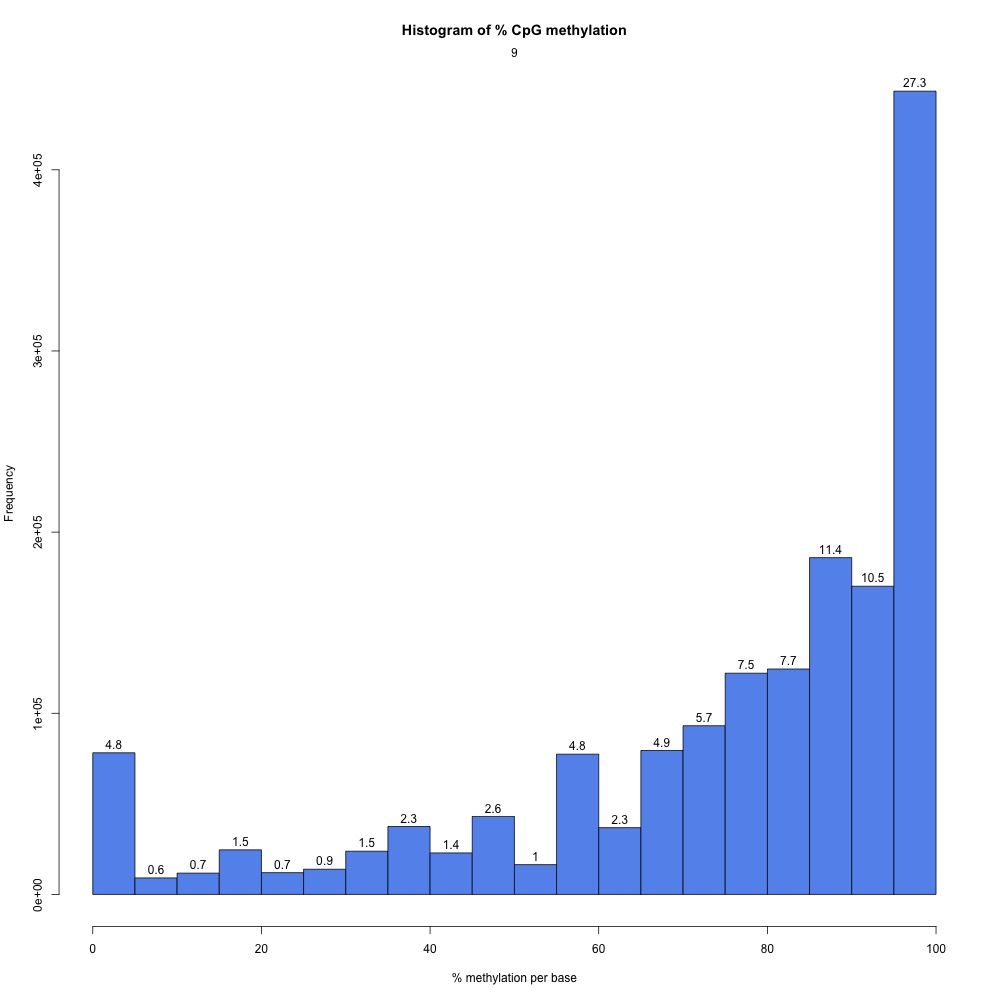
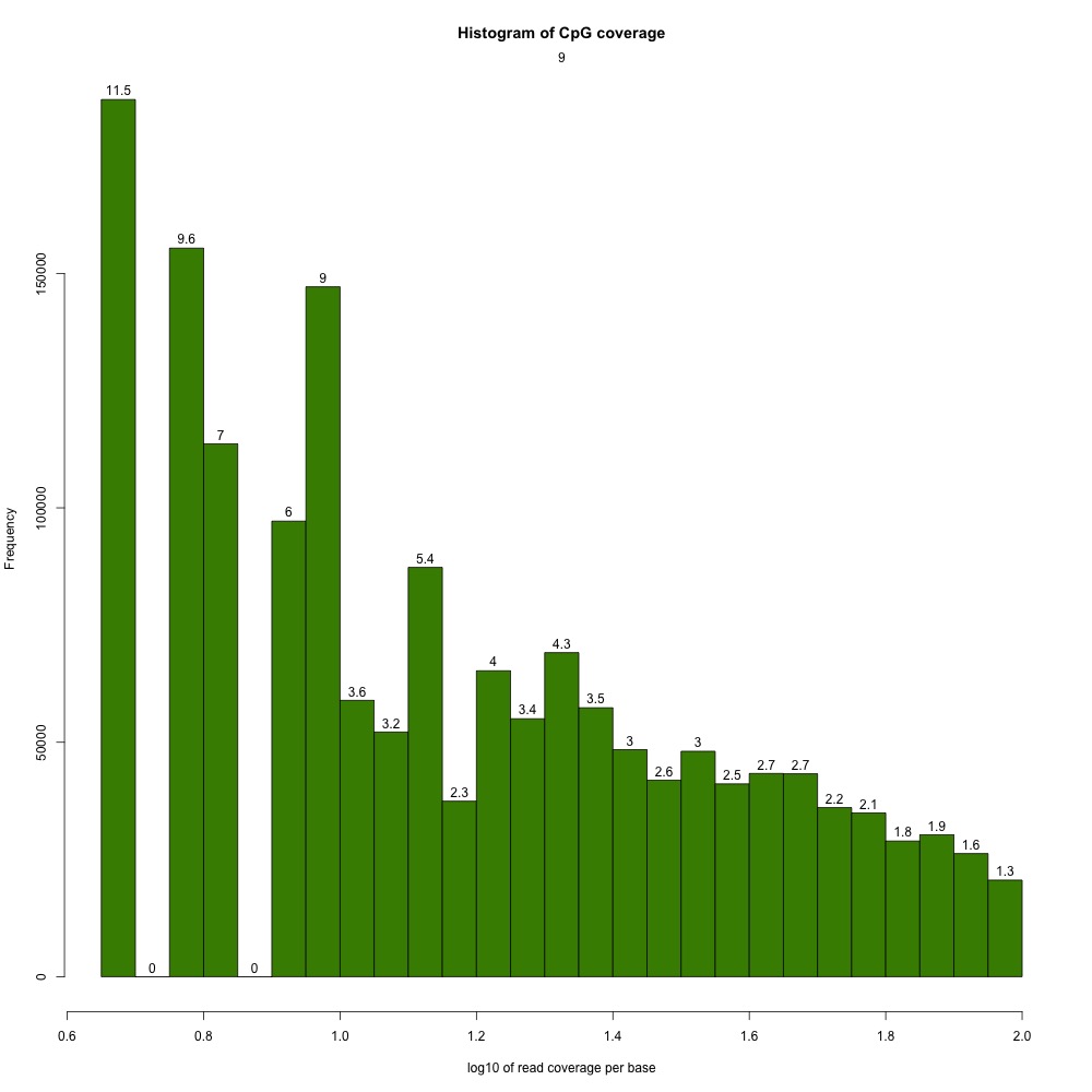
Figures 2-3. Sample 9 %CpG and CpG coverage plots.

I also evaluated clustering for the filtered 5x coverage data.

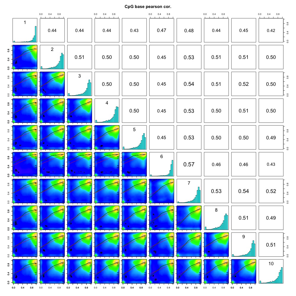
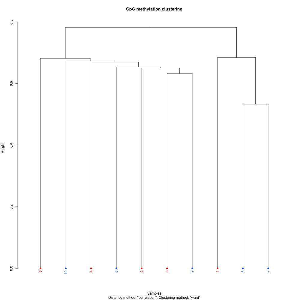
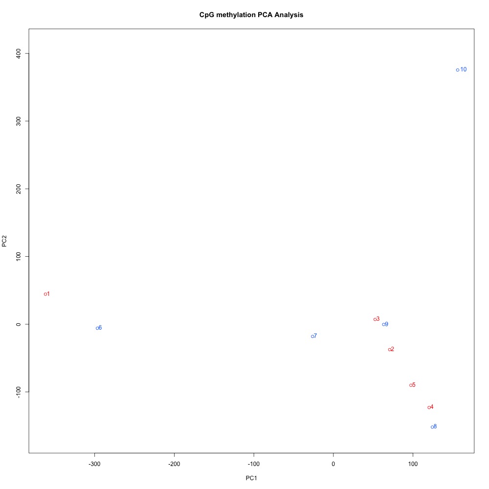
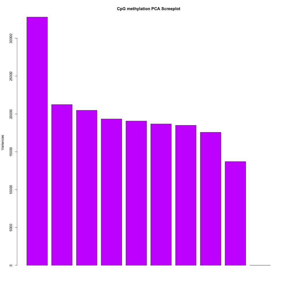
Figures 4-7. Correlation plot, full sample clustering, full sample PCA, and scree plot for filtered 5x coverage data.

Finally, I identified DML. I got 598 DML, which still doesn’t match Steve’s result. It’s also less DML than I had before. I exported the data to this file. I thought it may have been a versioning issue, so I updated R and methylKit. I still ended up with 598 DML, so there must be something else going on.

Recharacterizing DML locations

I characterized genomic locations for my new DML set. As expected, the majority of overlaps, 368 (61.5%), were with exons. There were also 191 DML (31.9%) that overlapped with introns. Transposable elements overlapped with 57 DML (9.5%) when all speices were used, and 39 DML (6.5%) when only C. gigas was used. Putative promoter regions overlapped with 67 DML (11.2%). There were also 20 DML (3.3%) with no overlaps with exons, introns, transposable elements (all), and putative promoter regions.

Checking read calculations

I initially listed 190 million reads mapping back to the C. virginica genome from my samples, but this was a much higher rate than any of the mapping efficiencies I had in a sample. In this Jupyter notebook, I recalculated the number of mapped reads. I pulled out mapping efficiency, then the number of sequence pairs analyzed, for each sample. I then used a series of bash commands to isolate mapping efficiency percentages and multiply them by pairs analyzed:

#Isolate mapping efficiency percentages (remove % from the end)
#Save new document
!cut -f2 2019-03-17-Mapping-Efficiency.txt | cut -c1-4 \
| paste 2019-03-17-Mapping-Efficiency.txt -> 2019-03-17-Mapping-Efficiency-Percents-Included.txt

#Divide percentages by 100
#Save new document
!awk -v c=100 '{ print $3/c}' 2019-03-17-Mapping-Efficiency-Percents-Included.txt \
| paste 2019-03-17-Mapping-Efficiency-Percents-Included.txt -> 2019-03-17-Mapping-Efficiency-Divided-Percents.txt

#Isolate pairs analyzed
#Save in new document with divided percents
!cut -f2 2019-03-17-Pairs-Analyzed.txt \
|paste 2019-03-17-Mapping-Efficiency-Divided-Percents.txt -> 2019-03-17-Pairs-Analyzed-and-Mapping-Efficiency.txt

#Mulitply percentage mapped and pairs analyzed columns to obtain mapped reads
!awk '{ print $3, $6, $5*$6}' 2019-03-17-Pairs-Analyzed-and-Mapping-Efficiency.txt \
> 2019-03-17-Mapped-Reads.txt

#Sum the contents of the third column ($3) to obtain the total number of paired-end reads that mapped to the genome.
!cat 2019-03-17-Mapped-Reads.txt | awk '{ sum+=$3} END {print sum}'

I found 136,186,380 paired-end reads had mapped to the genome, or 49.4%. This makes much more sense with my mapping efficiencies.

Additionally, I revised my paper to include a statement about the number of loci with 5x coverage, instead of 1x coverage. In this Jupyter notebook, I set a 5x coverage threshold and counted CpGs. I have data for 911,159 CpGs, which is 62.4% of CpGs in the genome.

Updating gannet

Since I generated a lot analytical output, I decided to upload the current version of my repository to gannet. It can be found at this link. As I continue to finalize analyses, I’ll probably keep updating the same repository link so I don’t end up with 13 different repository versions over the course of a week.

New paper repository

Steven also created a new paper repository in the NSF E20 organization. I’ll update the repository with polished scripts to ensure Katie and Alan can reproduce my results. I cross-referenced my scripts, R Markdown file, and Jupyter notebooks with my current methods and the draft paper. I also organized the files in the sequence they should be used and added short descriptions in the README.

Going forward

1. Check that I identified methylated CpGs correctly
2. Chi-squared tests for DML distribution
3. Describe (somehow) genes with DML in them
4. Figure out what’s going on with the gene background
5. Figure out what’s going on with DMR
6. Work through gene-level analysis
7. Update paper repository
8. Start writing the discussion
9. Draft timeline to finish the paper by the end of the month