Exon methylation and expression

I’m continuing the work we started at CEABiGR by playing around with an R package called mixOmics. My goal is to conduct an sparse Partial Least Squares (sPLS) analysis with exon expression and methylation data to understand correlations between the datasets, and identify individual exons with expression or methylation patterns driving the correlations. I’m working in this R Markdown script and following the code from this mixOmics handbook section.

Filtering data

Based on the sPLS trials I did at FHL, I knew I needed to filter the expression and methylation data not just for the statistical element, but because I couldn’t run the package with such large datasets! I started by filtering out missing values. If any sample was missing data for a specific exon, then that exon was removed from the dataframe. This wasn’t enough to be able to run the analysis. Similar to what Katherine did for the mQTL analysis, I removed exons that were not variable between sample by finding the range of percent methylation for an exon, and removing it from the dataset if the range < 10% methylated. This is the same cutoff we used to define lowly methylated loci.

#Transpose methylation data
#Remove rows with missing data
#Rowwise range operation
#Remove rows without big differences in exon methylation
exonMethylationFilt <- exonMethylationMod %>%
  t(.) %>%
  as.data.frame(.) %>%
  rownames_to_column("exon") %>%
  drop_na(.) %>%
  rowwise() %>%
  mutate(range = max(c_across(where(is.numeric))) - min(c_across(where(is.numeric)))) %>%
  column_to_rownames("exon") %>%
  filter(., range > 10) %>%
  select(., !range) %>%
  t(.) %>%
  as.data.frame(.)
head(exonMethylationFilt) #Confirm formatting
sum(is.na(exonMethylationFilt)) #Confirm there are no NAs
ncol(exonMethylationFilt) #Number of exons remaining

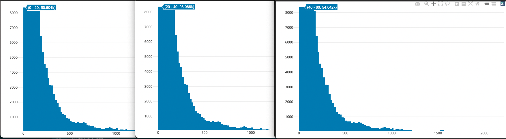
For the eQTL analysis, Laura removed low frequency genes (sum of expression data < 10). Instead of using this cutoff, I plotted an interactive histogram of the range in expression values across all samples for a specific exon with plot_ly:

exonExpressionHist <- exonExpressionMod %>%
  t(.) %>%
  as.data.frame(.) %>%
  drop_na(.) %>%
  rowwise() %>%
  summarise(range = max(c_across(where(is.numeric))) - min(c_across(where(is.numeric)))) #Calculate the range of exon expression values across each sample

plot_ly(x = exonExpressionHist$range, type = "histogram") #Interactive plot of exon expression value ranges

I zoomed into the plot to identify how many counts were in the lowest bins: 0-20, 20-40, and 40-60. Based on these counts, I decided to remove exons with range values < 20. P.S. plot_ly is super cool for exploratory analyses!

#Transpose expression data
#Remove rows with missing data
#Rowwise range operation
#Remove rows without big differences in exon expression
exonExpressionFilt <- exonExpressionMod %>%
  t(.) %>%
  as.data.frame(.) %>%
  rownames_to_column("exon") %>%
  drop_na(.) %>%
  rowwise() %>%
  mutate(range = max(c_across(where(is.numeric))) - min(c_across(where(is.numeric)))) %>%
  column_to_rownames("exon") %>%
  filter(., range > 20) %>%
  select(., !range) %>%
  t(.) %>%
  as.data.frame(.)
head(exonExpressionFilt) #Confirm formatting
sum(is.na(exonExpressionFilt)) #Confirm there are no NAs
ncol(exonExpressionFilt) #Number of exons remaining

Full sample sPLS

I ran the default sPLS parameters with the filtered exon expression and methylation datasets:

exonResult.spls <- spls(X = exonMethylationFilt, Y = exonExpressionFilt,
                        keepX = c(25, 25), keepY = c(25,25)) #Run SPLS

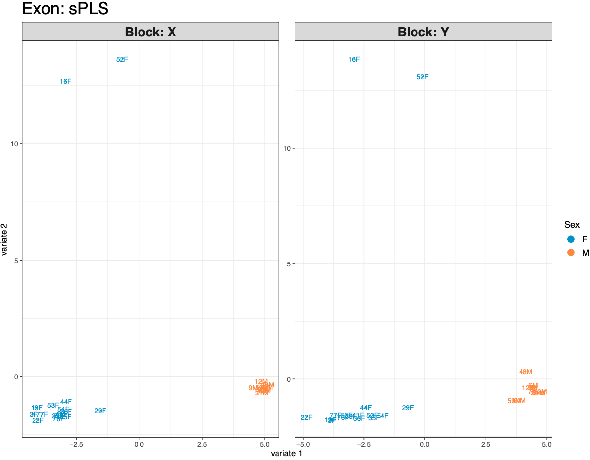
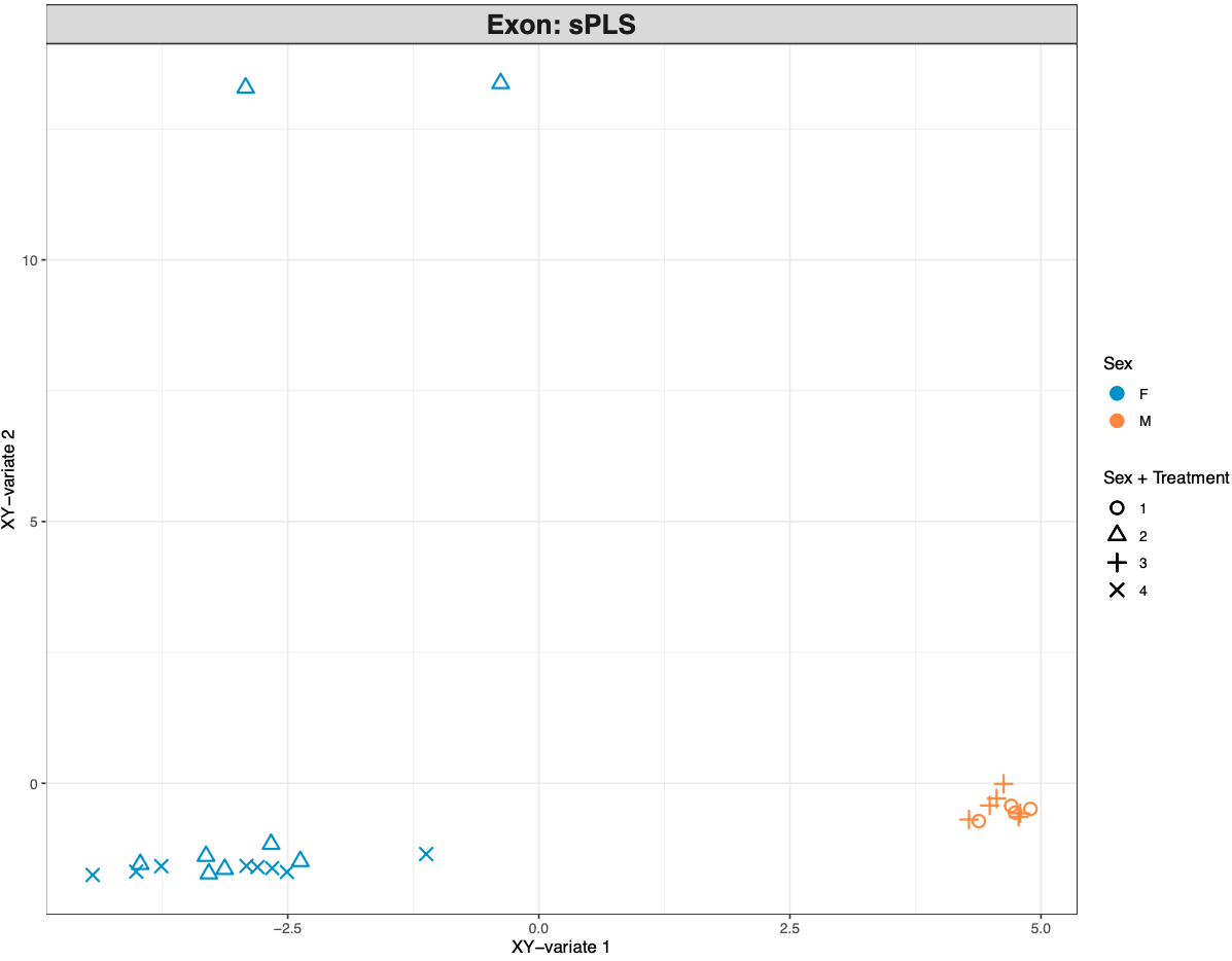
Figures 1-2. sPLS sample plots for all samples.

Based on the subset I ran prior to filtration during the workshop, I suspected I needed to separate male and female data. The plots confirm this, with male and female data separating very clearly. Samples 16F and 52F are also separating from the rest of the female samples, which is interesting and may be something to deal with in the future. There’s some slight separation of low and ambient pH samples, which I suspect will be clearer when I run sex-specific analyses. Now that I’ve run the full sample sPLS, I have the evidence I need to separate samples by sex!

Going forward

1. Revise with new expression data from Ariana
2. Tune SPLS parameters
3. Run sex-specific SPLS
4. Identify drivers