Survival analysis

Time to get cranking on analyzing my C. maenas data from last summer! My goal is to analyze all data except for the metabolomics data before I leave for India. This will help me understand which temperature treatments and sampling points may be useful for this summer’s experiment with West Coast crabs. I decided to knockout the lowest hanging fruit: comparing C. maenas survival across temperatures.

I knew I needed to make Kaplan-Meier curves to visualize survivorship across experimental days, but other than that I had no idea what I was doing. I found this guide to survival analysis in R which was extremely helpful! I also got some insight into survival analysis from Dr. Lindsay Alma (my friends are so cool and official). The first thing I needed to was format my dataframe. I had a spreadsheet that tracked the number of crabs alive in a tank every day of the experiment. I needed to convert this into a long dataframe, where each row had time (days until death), status (1 = event, 0 = censored), treatment (13C = ambient, 5C = cold, 3OC = hot) columns. To do this, I used a series of tidyverse functions to count the number of crabs that died each day, then duplicated rows by the number of crabs that died using uncount. I also had to indicate which crabs were censored and which actually died. For survival analysis, censoring means the individiual left the experiment without dying (the “event”). When I sampled crabs for metabolomics, they were censored. This is important to include since survival probabilities are calculated taking these crabs into consideration for the duration they were actually present in the experiment. When I first tried the survival analysis, I made two mistakes:

1. Not including information for crabs censored at the end of the experiment (aka crabs that were still alive at the end), which skewed the curves and survival probabilities
2. Using treatment as a continuous number scale instead of a factor, which didn’t let me understand pairwise differences between the hot or cold treatment and the control.

My final code to modify my dataframe was as follows. First I created a wide dataframe with mortality data instead of survival data:

mortalityData <- survivalData[NA,] %>%
  mutate(., tank = survivalData$tank) %>%
  mutate(., "1" = rep(0, times = 6)) %>%
  mutate(., "23" = survivalData$`22`) #Create an empty dataframe with the same structure as survivalData. Copy tank column into the new dataframe. First day had 0 mortalities. Add a column with remaining live crabs as day 23.
rownames(mortalityData) <- rownames(survivalData) #Use the same row names
for (i in 3:23) {
  mortalityData[,i] <- survivalData[,(i-1)] - survivalData[,i]
} #Subtract the number of alive crabs each day from how many there were the day before to calculate how many died each day.

Then I converted my mortality data into a long format with the necessary columns for the survival package:

mortalityDataLong <- mortalityData %>%
  pivot_longer(., cols = -tank, names_to = "day", values_to = "num_died") %>%
  mutate(status = case_when(day == 4 | day == 23 ~ 0,
                            day != 4 | day == 23 ~ 1)) %>%
  mutate(time = as.numeric(day)) %>%
  select(., -day) %>%
  filter(., num_died != 0) %>%
  uncount(., weights = num_died) %>%
  mutate(., treatment = case_when(tank == "T1" | tank == "T4" ~ "13C",
                                  tank == "T2" | tank == "T5" ~ "5C",
                                  tank == "T3" | tank == "T6" ~ "30C")) %>%
  select(., -tank) %>%
  mutate(., time = replace(time, time == 23, 22))
#Pivot the dataframe longer, using former column names as experimental day indication and values as number of crabs that died each day. Use case_when to assign status information (0 = censored/sampled, 1 = mortality) based on day (day 4 = 3 crabs sampled for metabolomics, day 23 = end of experiment). Create a column "time" which is a numeric version of day, then remove day. Create a duplicate row for each crab that died using uncount. Use case_when to assign treatment information to each tank and remove the tank column. Replace time = 23 with 22, since 23 was used to easily separate censored and uncensored crabs.

Once I had my formatted dataframe, I used Surv to create a survival object, which I then called within survdiff to run a non-parametric Kaplan-Meier survival analysis:

mortalityDataLong %>%
  survdiff(Surv(time, status, type = "right") ~ treatment, data = .) #Use a log-rank test to compare temperature treatments. Significant effect of treatment on mortality (Chisq= 18.7  on 2 degrees of freedom, p= 9e-05)

This test showed that overall, survival probability differed between treatments. I then used a Cox proportional hazards regression model to understand if the hazard of death was significantly different for the 30ºC or 5ºC versus the 13ºC control:

coxModel <- mortalityDataLong %>%
  coxph(Surv(time, status, type = "right") ~ treatment, data = .) #Use a Cox regression model to investigate survival differences by treatment.
coxModel #Significant difference between 13 and 30, not between 13 and 5

#                 coef exp(coef) se(coef)     z       p
# treatment30C 2.11819   8.31608  0.76095 2.784 0.00538
# treatment5C  0.03381   1.03439  1.00001 0.034 0.97303
#
# Likelihood ratio test=16.69  on 2 df, p=0.0002372
# n= 86, number of events= 17

summary(coxModel) #Confidence interval information for each treatment as compared to the base condition (13)

#              exp(coef) exp(-coef) lower .95 upper .95
# treatment30C     8.316     0.1202    1.8715    36.952
# treatment5C      1.034     0.9668    0.1457     7.343

The exp(coeff) is the hazard ratio (HR), where a HR > 1 means there is an increased chance of death each day of the experiment when compared to the contro, with the opposite being true for HR < 1. There was an 8.32-fold increase in the chance of death for the 30ºC versus the 13ºC treatment, but no significant differences in HR between the 5ºC and 13ºC.

I used Kaplan-Meier curves to visualize differences in survival probability over the course of the experiment. I distinguished between treatments using different colors and linetypes, and used annotate to add statistical output to the plot.

mortalityDataLong %>%
  survfit2(Surv(time, status, type = "right") ~ treatment, data = .) %>%
  ggsurvfit(linewidth = 1, linetype_aes = TRUE) +
  scale_color_manual(values = c(plotColors[2], plotColors[1], plotColors[3]),
                     labels = c("13", "30", "5"),
                     name = "Treatment (ºC)") +
  scale_linetype_manual(values = c(1, 6, 4),
                        labels = c("13", "30", "5"),
                        name = "Treatment (ºC)") +
  scale_x_continuous(breaks = seq(0, 22, 2)) +
  scale_y_continuous(limits = c(0, 1), breaks = seq(0, 1, 0.2)) +
  labs(x = "Days", y = "Overall Survival Probality") +
  annotate(geom = "text", x = 2, y = 0.2,
           label = expression(paste(bolditalic("Overall: "), Chi^2, " = 18.7, p = 9 x ", 10^-5)),
           hjust = 0) +
  annotate(geom = "text", x = 2, y = 0.16,
           label = expression(paste(bolditalic("13ºC vs. 30ºC: "), "HR = 8.32, p = 0.005")),
           hjust = 0) +
  annotate(geom = "text", x = 2, y = 0.12,
           label = expression(paste(bolditalic("13ºC vs. 5ºC: "), "HR = 1.03, p = 0.97")),
           hjust = 0) +
  theme_classic(base_size = 15) #Plot KM curves based on the Surv object analyzing survival time by treatment, with "right" indicating the kind of censoring (samples still alive at the end of the experiment were "right" censored). Customize line width, line type, colors, legend, axes, and labels. Add annotations for statistics. Use default R plotting theme with a base font size of 15.

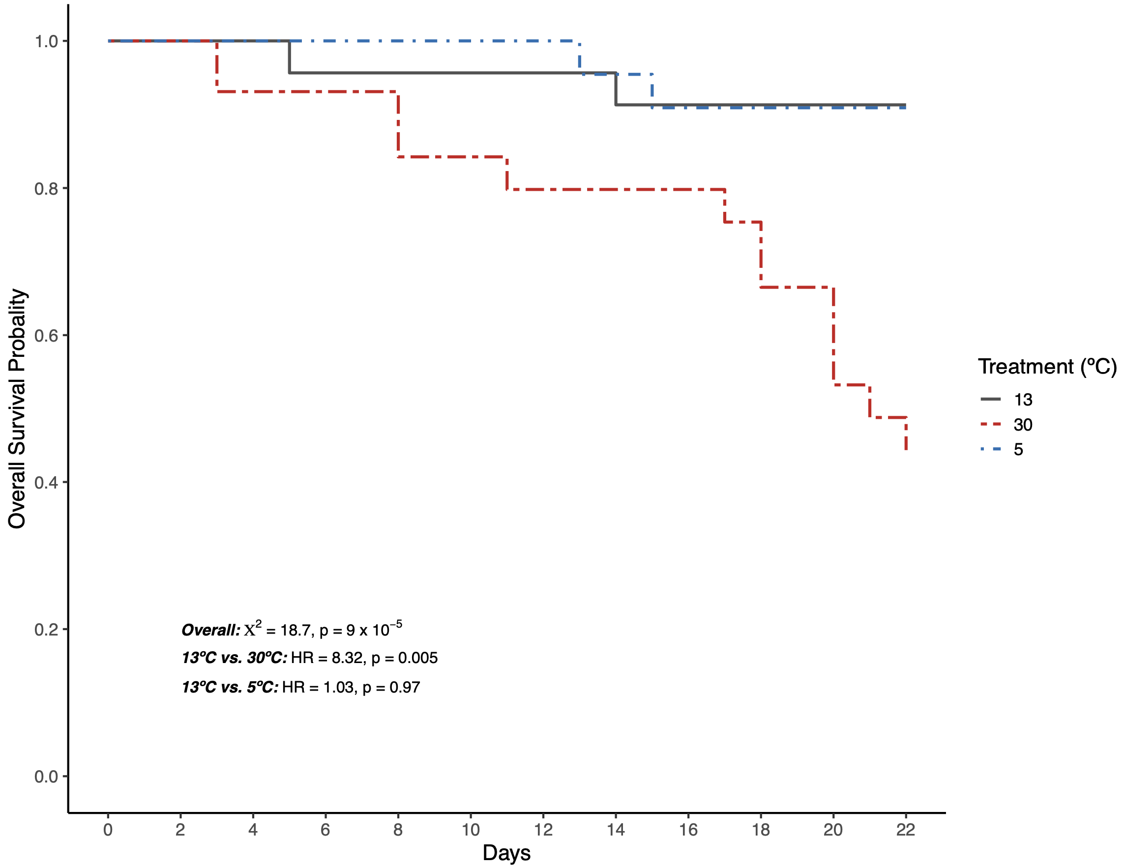
Figure 1. Kaplan-Meier curves for overall survival probability of crabs during the experiment

Next up, finishing the demographic data analysis!

Going forward

1. Test waterproof labeling system on a few crabs
2. Order extraction materials
3. Order 2023 experiment materials
4. Finalize demographic data analysis
5. TTR analysis
6. Update methods
7. Update results
8. Respirometry analysis