
Green Crab Experiment Part 16
Time-to-right analysis
Next physiology analysis: time-to-right! I wanted to understand how the righting response changed with temperature and over time. Based on conversations with Carolyn, I first looked through the literature to see how similar data were analyzed:
Cuculescu et al. 1998: The data were analyzed using one-way ANOVA, combined with the “least significant difference” range test, when more than two groups were compared.
Hopkin et al. 2006: Differences between the mean seasonal CTMax values in winter and summer for each species were assessed for significance using Student’s t-tests (one-tailed). One-tailed tests were selected since it is reasonable to predict a higher CTMax in the summer than in the winter in temperate latitudes.
Jost et al. 2012: Data were analyzed by a linear regression analysis to test whether the slope of the resulting regression line was significantly different from zero and whether significant differences between slopes exist (GraphPad InStat). Data were also analyzed for breakpoints using a Q-BASIC program for the identification of critical points (Yeager & Ultsch 1989). A p < 0.05 was considered significant. If no linear regression could be fit through the data and no breakpoint could be identified, we performed a 2-way ANOVA and a Tukey post hoc test to test for significant differences.
Coyle et al. 2019: Two models were run. The first included all reproductive, ecological and morphological variables (sex, morph color type, number of legs, sampling location and carapace width) to determine whether any of these variables were associated with the righting response. The results of this model were used to select a smaller set of relevant variables for the final model, which included sex, sampling location and three genetic terms for mitochondrial and nuclear variation.
Blakslee et al. 2021: Time-to-right data were log transformed for normality and analysed using an ANOVA with sex, size, and treatment as fixed effects and time-to-right as response variable.
Overall, most studies use some form of ANOVA or linear model to analyze differences in time-to-right. I decided on a two-prong approach:
- How does time-to-right change over time and with temperature?
- How do time and temperature impact whether or not a crab exhibited the righting response within a given threshold?
Initial visualizations
But first…visualizations! I decided to plot the data to see if there were any relationships or tests I wanted to try that I was not initially aware of. I first formatted the data, adding various columns for day, treatment, a binary for whether or not crabs were missing legs, an index for length and width, removing outliers (91 s), and averaging TTR across the three trials per crab and across treatments.
modTTR <- rawTTR %>%
  dplyr::select(., -c(sampling.ID, notes, probe.number)) %>%
  mutate(., day = case_when(date == "7/8/2022" ~ 4,
                            date == "7/12/2022" ~ 8,
                            date == "7/15/2022" ~ 11,
                            date == "7/19/2022" ~ 15,
                            date == "7/22/2022" ~ 18,
                            date == "7/26/2022" ~ 22)) %>%
  mutate(., treatment = case_when(treatment.tank == "1" | treatment.tank == "4" ~ "13C",
                                  treatment.tank == "2" | treatment.tank == "5" ~ "5C",
                                  treatment.tank == "3" | treatment.tank == "6" ~ "30C")) %>%
  mutate(., size = carapace.width/carapace.length) %>%
  mutate(., missing.legs = case_when(number.legs < 10 ~ "Y",
                                     number.legs == 10 ~ "N")) %>%
  mutate(., trial.1 = na_if(trial.1, 91.00)) %>%
  mutate(., trial.2 = na_if(trial.2, 91.00)) %>%
  mutate(., trial.3 = na_if(trial.3, 91.00)) %>%
  rowwise(.) %>%
  mutate(., TTRavg = mean(c(trial.1, trial.2, trial.3), na.rm = TRUE)) %>%
  filter(., is.na(TTRavg) == FALSE) %>%
  mutate(., TTRSE = std.error(c(trial.1, trial.2, trial.3), na.rm = TRUE)) %>%
  filter(., is.na(TTRSE) == FALSE) %>%
  group_by(., day, treatment) %>%
  mutate(., TTRavgFull = mean(TTRavg)) %>%
  mutate(., TTRSEFull = std.error(TTRavg)) %>%
  mutate(., TTRavgFullLow = TTRavgFull - TTRSEFull) %>%
  mutate(., TTRavgFullHigh = TTRavgFull + TTRSEFull) %>%
  ungroup(.) #Remove sampling ID and notes columns. Add new column with day information. Add new column with treatment information. Create a a new column that with an index for width/length. Create new column as a binary for whether or not crabs are missing legs. Change all 91 to NA, calculate average and SE using data from the three TTR trials using rowwise operations, and remove rows where TTRavg | TTRSE = NA.  Calculate average and SE for all samples in a treatment for each day. Add/subtract TTRSEFull to/from TTRavgFull to get bounds. Ungroup.
I then plotted TTR averaged across the three trials for each crab veruss day, coloring by treatment, sex, tank, integument color, number of legs, weight, and size. All the plots can be found here. I didn’t see any variables jumping out as influencing TTR aside from treatment (so that’s good).
Differences in time-to-right
To tackle the first question, I used an ANOVA to understand differences in the log-transformed average time-to-right in seconds by treatment, time, and other demographic data similar to Blakeslee et al. 2021. The decision to use an ANOVA took a bit of time. Initially, I used a linear model, but when I looked at the residuals I saw vertical lines in my residual plot. I asked ChatGPT what this meant, and it suggested that the discretization could be because I’m using several discrete, or categorical, explanatory variables that do not capture the full variation in the model. I engaged in a back-and-forth with the AI trying to figure out a better approach to analyze the data. It initially suggested using a glm with a logarithmic link function. When I tried this in R, I got a new error: Error: Error in eval(family$initialize): cannot find valid starting values: please specify some. Turns out I needed to provide initial model estimates prior to using this method. I didn’t feel comfortable doing a supervised analysis, so I pivoted to the ANOVA. Interestingly, the residual plot shows less discretization when I use an ANVOA instead of a glm with stepwise deletion! With both the initial GLM and the final ANOVA, treatment was significant, but day was marginally significant:
TTRmodel <- aov(log(TTRavg) ~ treatment + day + treatment*day + as.factor(sex) + as.factor(integument.color) + size + weight + as.factor(missing.legs), data = modTTR) #ANOVA, with log(TTRavg) as the response variable, and treatment, day, the interaction between treatment and day, sex, integument color, size, weight, and whether or not a crab is missing legs as explanatory variables.
summary(TTRmodel) #Only treatment is significant
                             Df Sum Sq Mean Sq F value Pr(>F)
treatment                     2 183.51   91.75 194.880 <2e-16 ***
day                           1   1.29    1.29   2.735 0.0995 .
as.factor(sex)                1   0.26    0.26   0.562 0.4542
as.factor(integument.color)   6   0.56    0.09   0.197 0.9773
size                          1   0.78    0.78   1.656 0.1994
weight                        1   0.57    0.57   1.219 0.2706
as.factor(missing.legs)       1   0.27    0.27   0.563 0.4537
treatment:day                 2   0.67    0.34   0.715 0.4901
Residuals                   239 112.53    0.47
---
Signif. codes:  0 ‘***’ 0.001 ‘**’ 0.01 ‘*’ 0.05 ‘.’ 0.1 ‘ ’ 1
My ANOVA output table can be found here. I then conducted post-hoc tests to understand my results. I initially used TukeyHSD to run the post-hoc test, but I got an error. Again, I asked my new BFF ChatGPT to tell me how to analyze the data. Turns out the Tukey test was only appropriate when I had categorial data. I used the Tukey test for treatment, but then used a pairwise t-test to understand differences by day.
TukeyHSD(TTRmodel, "treatment", conf.level = 0.95) #Use TukeyHSD for categorical variables. Significant difference between all pairwise treatment comparisons.
Tukey multiple comparisons of means
    95% family-wise confidence level

Fit: aov(formula = log(TTRavg) ~ treatment + day + treatment * day + as.factor(sex) + as.factor(integument.color) + size + weight + as.factor(missing.legs), data = modTTR)

$treatment
              diff        lwr          upr     p adj
30C-13C -0.2602039 -0.5107776 -0.009630257 0.0397611
5C-13C   1.6562160  1.4135681  1.898863936 0.0000000
5C-30C   1.9164200  1.6632199  2.169620038 0.0000000
Based on the Tukey test output, there is a significant difference between the 5ºC and the other two treatments, where TTR is higher for the 5ºC treatment. There is also a significant difference between the 30ºC and 13ºC, with TTR for the 30ºC crabs being slightly lower. You can’t really see this when plotting because the numbers are so close together.
pairwise.t.test(x = log(modTTR$TTRavg), modTTR$day, p.adjust.method = "bonferroni") #Use pairwise t-test for quantitative variables. Marginal significance between days 4 and 11.
Pairwise comparisons using t tests with pooled SD

data:  log(modTTR$TTRavg) and modTTR$day

   4    8    11   15   18
8  1.00 -    -    -    -
11 0.10 0.17 -    -    -
15 1.00 1.00 1.00 -    -
18 1.00 1.00 1.00 1.00 -
22 1.00 1.00 0.26 1.00 1.00

P value adjustment method: bonferroni
Looking at the pairwise t-test output, the marginal significance in day is likely driven by the difference between day 11 and day 4 values. At day 11, there’s a huge drop in TTR for the 5ºC crabs, which then bumps up again day 15. Interestingly, I didn’t remove any outliers from day 11, so these are real measurements!
Threshold analysis
The last thing I wanted to do analytically is determine if there’s a difference in the proportion of crabs that righted within a specific threshold by day and treatment. The first thing I needed to do was pick a threshold. I asked ChatGPT how to find outliers, and one of its suggestions was to use a boxplot, since values are sorted into quantiles and identified as outliers if they do not fit those bounds. I was interested in upper outliers, since I have right-skewed data:
boxplot.stats(modTTR$TTRavg)$stats[5] #Use Tukey's method to identify upper bound of outliers
The upper bound was identified as ~9.2. I then added a column to my dataset with a binary for whether the crab righted within 9.2 seconds (1), or whether it did not (0). I used a binomial GLM to analyze my data, similar to Coyle et al. (2019).
TTRthreshModel2 <- glm(I(TTRthresh == 1) ~ treatment + day,
                       family = binomial(),
                       data = modTTR) #Run model selected by step with only significant terms
summary(TTRthreshModel2) #control vs. 5C significantly different, significant impact of day
Call:
glm(formula = I(TTRthresh == 1) ~ treatment + day, family = binomial(),
    data = modTTR)

Deviance Residuals:
    Min       1Q   Median       3Q      Max
-3.1050   0.1052   0.1538   0.2306   1.3181

Coefficients:
             Estimate Std. Error z value Pr(>|z|)
(Intercept)   3.23199    1.07231   3.014 0.002578 **
treatment30C -0.05435    1.42631  -0.038 0.969604
treatment5C  -3.99281    1.03994  -3.839 0.000123 ***
day           0.10898    0.03765   2.895 0.003794 **
---
Signif. codes:  0 ‘***’ 0.001 ‘**’ 0.01 ‘*’ 0.05 ‘.’ 0.1 ‘ ’ 1

(Dispersion parameter for binomial family taken to be 1)

    Null deviance: 192.64  on 254  degrees of freedom
Residual deviance: 124.54  on 251  degrees of freedom
AIC: 132.54

Number of Fisher Scoring iterations: 7
Based on the model output, a crab’s ability to right within 9.2 seconds depended on treatment and day, with a significant difference between the 13ºC and 5ºC treatments. Once again, I asked ChatGPT for an appropriate post-hoc test to use, but I decided against using a post-hoc test since I already had all of the information I needed.
Plotting my results
The last thing I did was plot my results! I plotted average TTR for each treatment across time, and included SE bars for each point and a horizontal line at the 9.2 second threshold I used in the above analysis. I contemplated adding an inset for 0-1.5 seconds, but even looking at that didn’t resolve the differences between the 13ºC and 30ºC visually.
modTTR %>%
  dplyr::select(., c(day, treatment, TTRavgFull, TTRavgFullLow, TTRavgFullHigh)) %>%
  distinct(.) %>%
  ggplot(., mapping = aes(x = day, y = TTRavgFull, color = treatment)) +
  geom_pointrange(aes(ymin = TTRavgFullLow,
                      ymax = TTRavgFullHigh),
                  size = 0.5, alpha = 0.75) +
  geom_line(y = boxplot.stats(modTTR$TTRavg)$stats[5], lty = 2, color = "black") +
  scale_x_continuous(name = "Day",
                     breaks = unique(modTTR$day),
                     limits = c(4, 22)) +
  scale_y_continuous(name = "Average Time-to-Right (s)",
                     breaks = c(0, seq(1, 5, 2), seq(5, 20, 5)),
                     limits = c(0, 17)) +
  scale_color_manual(values = c(plotColors[2], plotColors[1], plotColors[3]),
                     name = "Temperature (ºC)",
                     breaks = c("13C", "30C", "5C"),
                     labels = c("13", "30", "5")) +
  theme_classic(base_size = 15) #Plot average TTR and add lm fits without SE bars. Add vertical line for boxplot outlier threshold. Modify x-axis to only show experimental days where TTR was measured. Scale y axis to include 91 = indication that crabs did not right within 90 s. Assign colors to each treatment. Increase base font size.
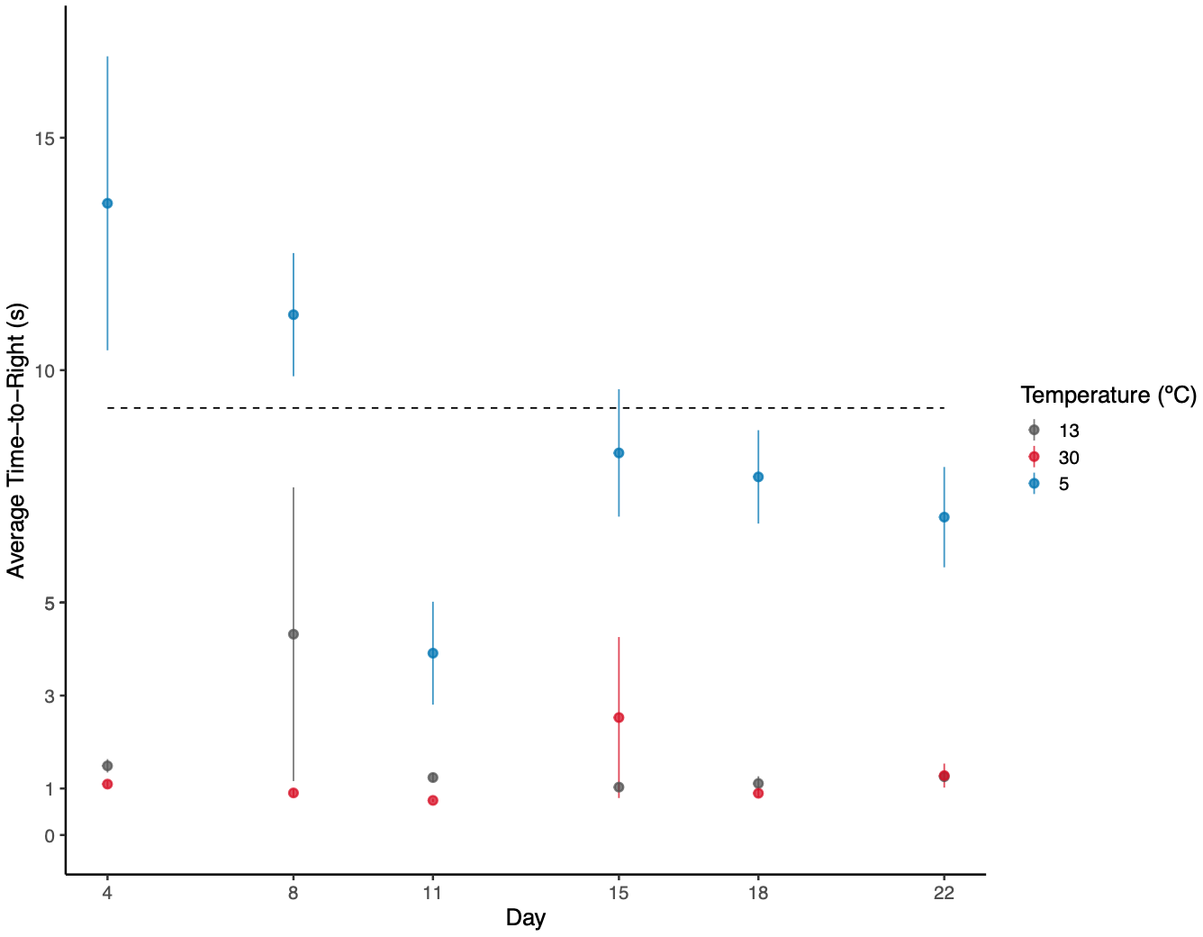
Figure 1. Average TTR for each treatment over time.
When looking at the figure, average TTR for the 5ºC slowly decreases over time, going under the 9.2 second threshold after day 11. There are very subtle differences between the 30ºC and 13ºC treatment, probably driven by the variation in day 8.
Going forward
- Test waterproof labeling system on a few crabs
- Order extraction materials
- Order 2023 experiment materials
- Finalize demographic data analysis
- Test formatting and analysis for one set of respirometry data
- Update methods
- Update results